Better Grafana Dashboards: Precise Prometheus Metrics Over Visual Illusion
Monitoring tools are indispensable to modern software development and cloud infrastructure. The pairing of Grafana as a visualization platform and Prometheus as a metrics backend is one of the most widely deployed in the field. It is remarkably easy to build good-looking graphs in Grafana—graphs that look excellent at first glance. All too often, though, these surface-level visualizations distort reality and lead to mistaken assumptions about system health. When critical patterns are lost in visual noise, troubleshooting quickly devolves into guesswork. This is precisely where we step in to create genuine transparency.
In this post, we show you how to get more out of your Grafana dashboards by avoiding the typical pitfalls of PromQL queries. We walk through practical solutions for precise visualizations. We also take a look at how AI tools can accelerate the initial setup of the underlying test infrastructure.
Efficient Infrastructure Setup with AI Assistance
To test visualization concepts on solid ground, you need a reliable and realistic data foundation. Typically, setting up such an environment by hand—a Prometheus instance connected to Grafana, plus representative test metrics—is time-consuming. This is exactly where AI assistants promise substantial efficiency gains.
Generating Test Data via Script
Rather than relying on trivial mock data, we use a Python script to generate OpenMetrics. The script produces historically backdated metrics that simulate typical load patterns—see the link to the GitHub repository in the references below.
This includes, for example, realistic business-hour peaks and deliberate error spikes. The result is a valid, true-to-life test environment that feeds directly into Prometheus and serves as the foundation for in-depth analysis.
LLM Performance on Infrastructure Code
When building out the container infrastructure, we compared several AI assistants, including Claude and other LLMs. Bootstrapping the basic docker-compose.yml files and baseline configurations worked out of the box.
That said, the models hit their limits on specific PromQL subtleties and more complex architectural questions. The takeaway is clear: AI is a powerful tool for setup work, but it is by no means a substitute for the deep architectural understanding an engineering team possesses.
Two Common Mistakes — and How to Fix Them
Even with the best infrastructure behind it, a dashboard lives and dies by the quality of its queries. Two pitfalls in particular deserve attention.
Spotting and Fixing the Percentile Trap
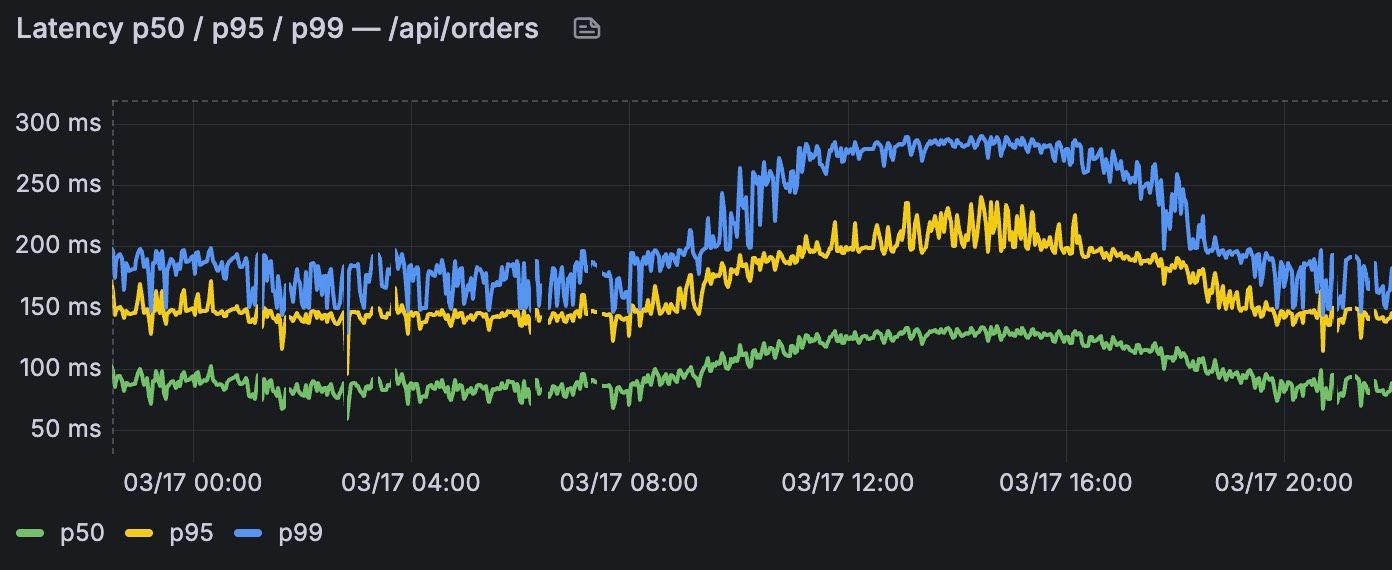
Latencies in Prometheus are typically instrumented as histograms—a decision made by the application that exposes the metrics. A histogram counts observed values into configurable buckets, where each bucket holds the count of all observations below a given upper bound (the le label). The concrete latency values of individual requests are lost in the process; what remains is only the information about how many requests fell into which bucket.
The PromQL function histogram_quantile() computes quantiles such as p95 or p99 from these bucket counters. Since the actual individual latencies are no longer known, the function has to make an assumption: it surmises that the observations within a bucket are uniformly distributed across its span, and interpolates linearly between the bucket boundaries.
This is exactly where the distortion comes in. Consider an example: the bucket 1s ≤ x < 5s contains three requests that, in reality, all came in at 1 second. The function arithmetically “invents” one request at 1s, one at 3s, and one at 5s — values that never actually occurred. The wider the buckets and the more uneven the real distribution within a bucket, the stronger the distortion. The result is a p99 that is systematically pulled toward the upper bucket boundaries and only inaccurately reflects the true latency.
The fix: Always complement your percentile graphs with a heatmap of the actual metric buckets. Grafana’s heatmap panel shows the “raw truth” of the histogram—how many requests there were in total at a given point in time; how they were distributed across the individual buckets; and which buckets are even defined in the histogram. Especially when investigating a spike in p99, the heatmap provides exactly the context that a sole percentile value cannot.
Mastering Time Ranges and Interpolation
This section addresses two related but technically distinct problems: choosing the right time window in PromQL queries, and the visual representation of the results in Grafana.
Problem 1: Range vector selectors and the query interval. In PromQL, functions like rate() or increase() operate on range vectors. A range vector—unlike an instant vector, which yields exactly one data point per series—is a matrix at its core: each row corresponds to a time series, each column to a point in time within a backward-looking window. It is produced by a range vector selector, written as a post fix of [5m] or [1h] of the metric name.
This window should never be hard-coded. Grafana provides the built-in variable $__rate_interval for exactly this purpose: it adjusts automatically to the current query interval—that is, the spacing between the data points being queried, which in turn depends on the selected time range. We therefore recommend the form rate(metric[$__rate_interval]).
In practice, however, the automatic behavior runs into limits. For large dashboard ranges, Grafana often computes values that are far too small for meaningful smoothing; and even with shorter ranges, you sometimes want to adjust the window manually to dampen noise deliberately or expose finer structures.
The fix: Introduce a custom dashboard variable—for example, an interval variable named “Min Range” with values like 1m, 5m, 10m, 15m, 30m, 1h, 3h, 6h, 12h, or 1d. The crucial point is to use this variable in the right way: not directly in the range vector selector, but in the panel setting Min step (or Min interval) of the Prometheus query. This sets a lower bound on the query interval Grafana computes. The built-in $__rate_interval and $__interval variables in the range vector selector adapt accordingly. Users gain control over granularity without touching the queries.
Problem 2: Visual interpolation between data points. Grafana’s time-series panel connects data points with straight lines by default (linear interpolation). This produces misleading diagonals between two measurements and suggests a gradual transition where in fact no data exists. Configure the line interpolation to Step before instead: the graph then shows horizontal steps and communicates visually and unambiguously that no new data was recorded between two
Conclusion
To make reliable operational decisions, monitoring data has to mirror reality as faithfully as possible. When you tune your Grafana dashboards along these lines, heatmaps supply the essential context behind percentile values, while clean interpolation and well-chosen dashboard variables proactively prevent visual misinterpretation.
AI tools dramatically accelerate the initial setup of the test infrastructure along the way, but human expertise remains indispensable for the analytical fine-tuning. In keeping with our guiding principle: Do it RIGHT. Only through technical precision do you create the transparency—and the trust in your cloud infrastructure—that you need.
Referenzen
- •GitHub Repo zu diesem Beitrag (Python Skript, Docker Setup, …)
- •Grafana Time Series Panel (Interpolationsmodi inkl. „Step before")
- •Grafana: Prometheus Template Variables (inkl.
$__rate_interval)
- •Prometheus: Histograms and Summaries (Best Practices, Quantil-Schätzfehler)
- •Prometheus: Querying Basics (Instant vs. Range Vector Selectors)